Python from q with embedPy
Use embedPy to call Python from PeachQ. This guide shows how to pass q vectors and tables to NumPy and pandas, let SciPy call a q function, and save a matplotlib chart. You'll install the dependencies and run each example in a local session.
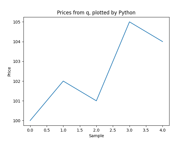
Generated by the recipe below from five example prices in a q vector.
Run it
Use Linux x86-64 with glibc, Bash, curl, tar, GNU sed, and Python 3 with
venv and pip available. This installs the Python packages in a local virtual
environment; it does not install Python itself. Start in a fresh directory.
Requires the Linux glibc build
This integration loads a shared library. Use PeachQ's Linux glibc build, available as the DuckDB/glibc download. The standard static Linux build cannot load shared libraries.
set -euo pipefail
mkdir peachq-python-demo && cd peachq-python-demo
mkdir peachq
curl -fL https://peachq.org/download/peachq-linux-x64-duckdb.tar.gz | tar -xz -C peachq
curl -fL https://github.com/KxSystems/embedPy/releases/download/1.5.0/embedPy_linux-1.5.0.tgz | tar -xz
python3 -m venv .venv
. .venv/bin/activate
python -m pip install "numpy<2" pandas scipy matplotlib

# Adapt the loader's two K composition expressions to q.
sed -i.before-peachq \
  -e "s|^k)c:.*|c:{{'[y;x]}/[reverse x]}|" \
  -e "s|^k)ce:.*|ce:{{'[y;x]}/[enlist,reverse x]}|" p.q

cat > chart.q <<'Q'
\l p.q
np:.p.import`numpy
prices:100 102 101 105 104f
show np[`:mean;<]prices
.p.import[`matplotlib;`:use;`Agg];
plt:.p.import`matplotlib.pyplot
plt[`:plot;til count prices;prices];
plt[`:title;"Prices from q, plotted by Python"];
plt[`:xlabel;"Sample"];
plt[`:ylabel;"Price"];
plt[`:savefig;"prices.png"];
plt[`:close][];
exit 0
Q
QHOME="$PWD" ./peachq/q chart.q
The mean is 102.4. Open prices.png to see the chart above.
Open an interactive session
Keep the virtual environment active. From the same directory:
QHOME="$PWD" ./peachq/q
Load the separately installed embedPy bridge once in each new q session, then
import NumPy. With this installation, calling .p.import does not automatically
load the external p.q:
0 1 2 3 4
hello from python
.p.import imports a Python module. The attribute selector `:arange
gets its arange function; < requests the result as q data. Lines starting
with p) execute Python in the same process.
Send q data to NumPy
Define a vector in q and pass it to Python functions:
Output:
102.4
1.854724
The vector crosses into Python as an argument, and both results return as q values. No CSV file or separate Python process is needed for these calls.
Group a q table with pandas
Create four example trades and build a pandas DataFrame from the table's column dictionary:
pd:.p.import`pandas
trades:([]sym:`AAPL`MSFT`AAPL`MSFT;size:10 20 30 40;price:100 200 102 201f)
df:pd[`:DataFrame.from_dict;flip trades]
df[`:groupby;`sym][`:sum][`numeric_only pykw 1b][`:to_dict][]`
Output:
|        | AAPL | MSFT |
| symbol |      |      |
|========|------|------|
| size   | 40   | 60   |
| price  | 202f | 401f |
The size totals are 40 for AAPL and 60 for MSFT. This example sums both numeric
columns to demonstrate the round-trip; the price sums are not a market-data
statistic. pykw supplies a Python keyword argument. The final backtick converts
the Python dictionary into q data.
Let SciPy call a q function
Fit the line y = a*x + b to five points. The model is a q function; SciPy calls
it during optimization:
Output:
2 1f
curve_fit returns fitted parameters and a covariance matrix; first selects
the parameters. The fitted slope is 2 and intercept is 1. Parentheses around a*x express the
intended formula under q's right-to-left evaluation.
The last argument, 1 0f, supplies initial guesses for the two parameters.
Keep it: supplying initial values avoids Python signature introspection for
the embedded q callback, as described
in the SciPy curve_fit reference.
Make the chart
Pass the original q vector to matplotlib and save an image:
.p.import[`matplotlib;`:use;`Agg];
plt:.p.import`matplotlib.pyplot
plt[`:plot;til count prices;prices];
plt[`:title;"Prices from q, plotted by Python"];
plt[`:xlabel;"Sample"];
plt[`:ylabel;"Price"];
plt[`:savefig;"prices.png"];
plt[`:close][];
Open prices.png in the current directory to see the chart at the top of this
article. The Agg backend saves the image without requiring a desktop window.
Download the complete q script. Save it in the demo directory, then run:
QHOME="$PWD" ./peachq/q embedpy-demo.q
The script prints each result and saves prices.png.
For more calling forms, see the embedPy user guide.
The loader adaptations retain the Apache-2.0 licence from KX embedPy.
What to keep in mind
You can now pass q data to Python, return results, fit a q callback with SciPy and save a chart with matplotlib.
- Shared libraries: use the glibc PeachQ package and a matching 64-bit Python.
- Loader adaptations: keep the two
sedreplacements in the setup. The loader's two K-mode composition expressions need their q equivalents. - NumPy: use
numpy<2with this embedPy release; these examples use NumPy 1.26.4. - Callbacks: give
curve_fitinitial parameter values for q functions; Python cannot infer their parameter names here.