Archive Page 5
March 30th, 2014 by Ryan Hamilton
In this tutorial we are going to recreate this example RSI calculation in q, the language of the kdb database.
The relative strength index (RSI) is a technical indicator used in the analysis of financial markets. It is intended to chart the current and historical strength or weakness of a stock or market based on the closing prices of a recent trading period. The RSI is classified as a momentum oscillator, measuring the velocity and magnitude of directional price movements. Momentum is the rate of the rise or fall in price.
The RSI computes momentum as the ratio of higher closes to lower closes: stocks which have had more or stronger positive changes have a higher RSI than stocks which have had more or stronger negative changes. The RSI is most typically used on a 14 day timeframe, measured on a scale from 0 to 100, with high and low levels marked at 70 and 30, respectively. Shorter or longer timeframes are used for alternately shorter or longer outlooks. More extreme high and low levels—80 and 20, or 90 and 10—occur less frequently but indicate stronger momentum.
.
Stock Price Time-Series Data
We are going to use the following example data, you can download the csv here or the excel version here.
| Date |
QQQQ Close |
Change |
Gain |
Loss |
Avg Gain |
Avg Loss |
RS |
14-day RSI |
| 2009-12-14 |
44.34 |
|
|
|
|
|
|
|
| 2009-12-15 |
44.09 |
-0.25 |
0.00 |
0.25 |
|
|
|
|
| 2009-12-16 |
44.15 |
0.06 |
0.06 |
0.00 |
|
|
|
|
| 2009-12-17 |
43.61 |
-0.54 |
0.00 |
0.54 |
|
|
|
|
| 2009-12-18 |
44.33 |
0.72 |
0.72 |
0.00 |
|
|
|
|
| 2009-12-21 |
44.83 |
0.50 |
0.50 |
0.00 |
|
|
|
|
| 2009-12-22 |
45.10 |
0.27 |
0.27 |
0.00 |
|
|
|
|
| 2009-12-23 |
45.42 |
0.33 |
0.33 |
0.00 |
|
|
|
|
| 2009-12-24 |
45.84 |
0.42 |
0.42 |
0.00 |
|
|
|
|
| 2009-12-28 |
46.08 |
0.24 |
0.24 |
0.00 |
|
|
|
|
| 2009-12-29 |
45.89 |
-0.19 |
0.00 |
0.19 |
|
|
|
|
| 2009-12-30 |
46.03 |
0.14 |
0.14 |
0.00 |
|
|
|
|
| 2009-12-31 |
45.61 |
-0.42 |
0.00 |
0.42 |
|
|
|
|
| 2010-01-04 |
46.28 |
0.67 |
0.67 |
0.00 |
|
|
RS |
RSI |
| 2010-01-05 |
46.28 |
0.00 |
0.00 |
0.00 |
0.24 |
0.10 |
2.39 |
70.53 |
| 2010-01-06 |
46.00 |
-0.28 |
0.00 |
0.28 |
0.22 |
0.11 |
1.97 |
66.32 |
| 2010-01-07 |
46.03 |
0.03 |
0.03 |
0.00 |
0.21 |
0.10 |
1.99 |
66.55 |
| 2010-01-08 |
46.41 |
0.38 |
0.38 |
0.00 |
0.22 |
0.10 |
2.27 |
69.41 |
| 2010-01-11 |
46.22 |
-0.19 |
0.00 |
0.19 |
0.20 |
0.10 |
1.97 |
66.36 |
| 2010-01-12 |
45.64 |
-0.58 |
0.00 |
0.58 |
0.19 |
0.14 |
1.38 |
57.97 |
| 2010-01-13 |
46.21 |
0.57 |
0.57 |
0.00 |
0.22 |
0.13 |
1.70 |
62.93 |
| 2010-01-14 |
46.25 |
0.04 |
0.04 |
0.00 |
0.20 |
0.12 |
1.72 |
63.26 |
| 2010-01-15 |
45.71 |
-0.54 |
0.00 |
0.54 |
0.19 |
0.15 |
1.28 |
56.06 |
| 2010-01-19 |
46.45 |
0.74 |
0.74 |
0.00 |
0.23 |
0.14 |
1.66 |
62.38 |
| 2010-01-20 |
45.78 |
-0.67 |
0.00 |
0.67 |
0.21 |
0.18 |
1.21 |
54.71 |
| 2010-01-21 |
45.35 |
-0.43 |
0.00 |
0.43 |
0.20 |
0.19 |
1.02 |
50.42 |
| 2010-01-22 |
44.03 |
-1.33 |
0.00 |
1.33 |
0.18 |
0.27 |
0.67 |
39.99 |
| 2010-01-25 |
44.18 |
0.15 |
0.15 |
0.00 |
0.18 |
0.26 |
0.71 |
41.46 |
| 2010-01-26 |
44.22 |
0.04 |
0.04 |
0.00 |
0.17 |
0.24 |
0.72 |
41.87 |
| 2010-01-27 |
44.57 |
0.35 |
0.35 |
0.00 |
0.18 |
0.22 |
0.83 |
45.46 |
| 2010-01-28 |
43.42 |
-1.15 |
0.00 |
1.15 |
0.17 |
0.29 |
0.59 |
37.30 |
| 2010-01-29 |
42.66 |
-0.76 |
0.00 |
0.76 |
0.16 |
0.32 |
0.49 |
33.08 |
| 2010-02-01 |
43.13 |
0.47 |
0.47 |
0.00 |
0.18 |
0.30 |
0.61 |
37.77 |
RSI Formulas
The formulas behind the calculations used in the table are:
- First Average Gain = Sum of Gains over the past 14 periods / 14.
- First Average Loss = Sum of Losses over the past 14 periods / 14
All subsequent gains than the first use the following:
- Average Gain = [(previous Average Gain) x 13 + current Gain] / 14.
- Average Loss = [(previous Average Loss) x 13 + current Loss] / 14.
- RS = Average Gain / Average Loss
- RSI = 100 – 100/(1+RS)
Writing the Analytic in q
We can load our data (rsi.csv) in then apply updates at each step to recreate the table above:
Code kindly donated by Terry Lynch
Rather than create all the intermediate columns we can create a calcRsi function like so:
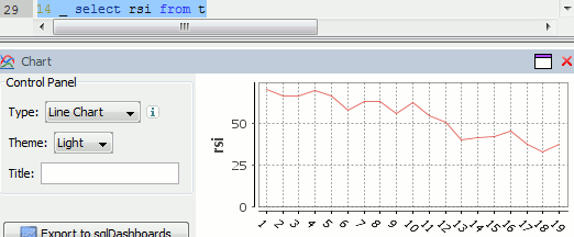
Finally we can visualize our data using the charting functionality of qStudio (an IDE for kdb):
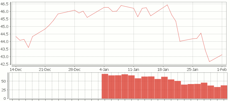
RSI Relative Strength Index stock chart for QQQQ created using qStudio
Or to plot RSI by itself (similar to original article
Writing kdb analytics such as Relative Strength Index is covered in our kdb training course, we offer both public kdb training courses in New York, London, Asia and on-site kdb courses at your offices, tailored to your needs.
March 29th, 2014 by Ryan Hamilton
Let’s look at how to write moving average analytics in q for the kdb database. As example data (mcd.csv) we are going to use stock price data for McDonalds MCD. The below code will download historical stock data for MCD and place it into table t:
Simple Moving Average
The simple moving average can be used to smooth out fluctuating data to identify overall trends and cycles. The simple moving average is the mean of the data points and weights every value in the calculation equally. For example to find the moving average price of a stock for the past ten days, we simply add the daily price for those ten days and divide by ten. This window of size ten days then moves across the dates, using the values within the window to find the average. Here’s the code in kdb for 10/20 day moving average and the resultant chart.
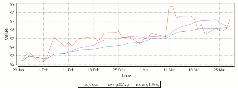
Simple Moving Average Stock Chart Kdb (Produced using qStudio)
What Exponential Moving Average is and how to calculate it
One of the issues with the simple moving average is that it gives every day an equal weighting. For many purposes it makes more sense to give the more recent days a higher weighting, one method of doing this is by using the Exponential Moving Average. This uses an exponentially decreasing weight for dates further in the past.The simplest form of exponential smoothing is given by the formula:

where α is the smoothing factor, and 0 < α < 1. In other words, the smoothed statistic st is a simple weighted average of the previous observation xt-1 and the previous smoothed statistic st−1.
This table displays how the various weights/EMAs are calculated given the values 1,2,3,4,8,10,20 and a smoothing factor of 0.7: (excel spreadsheet)
| Values |
EMA |
|
Power |
Weight |
Power*Weight |
|
EMA (text using previous value) |
| 1 |
1 |
|
6 |
0.0005103 |
0.0005103 |
|
1 |
| 2 |
1.7 |
|
5 |
0.001701 |
0.003402 |
|
(0.7*2)+(0.3*1) |
| 3 |
2.61 |
|
4 |
0.00567 |
0.01701 |
|
(0.7*3)+(0.3*1.7) |
| 4 |
3.583 |
|
3 |
0.0189 |
0.0756 |
|
(0.7*4)+(0.3*2.61) |
| 8 |
6.6749 |
|
2 |
0.063 |
0.504 |
|
(0.7*8)+(0.3*3.583) |
| 10 |
9.00247 |
|
1 |
0.21 |
2.1 |
|
(0.7*10)+(0.3*6.6749) |
| 20 |
16.700741 |
|
0 |
0.7 |
14 |
|
(0.7*20)+(0.3*9.00247) |
To perform this calculation in kdb we can do the following:
(This code was originally posted to the google mail list by Attila, the full discussion can be found here)
This backslash adverb works as
The alternate syntax generalizes to functions of 3 or more arguments where the first argument is used as the initial value and the arguments are corresponding elements from the lists:
Exponential Moving Average Chart
Finally we take our formula and apply it to our stock pricing data, allowing us to see the exponential moving average for two different smoothing factors:
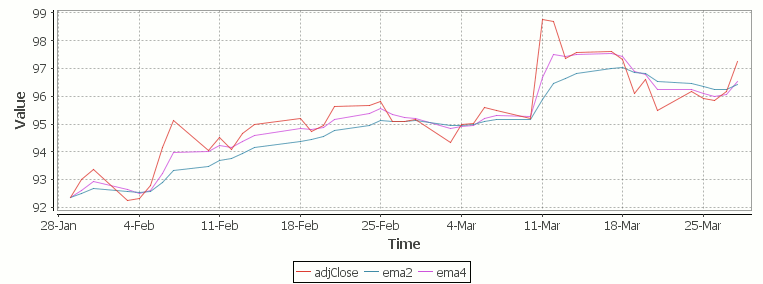
Exponential Moving Average Stock Price Chart produced using qStudio
As you can see with EMA we can prioritize more recent values using a chosen smoothing factor to decide the balance between recent and historical data.
Writing kdb analytics such as Exponential Moving Average is covered in our kdb training course, we regularly provide training courses in London, New York, Asia or our online kdb course is available to start right now.
December 15th, 2013 by Ryan Hamilton
In a previous post I looked at using the monte carlo method in kdb to find the outcome of rolling two dice. I also posed the question:
How can we find the value of Pi using the Monte Carlo method?
If we randomly chose an (x,y) location, we could calculate the distance of that points location ( sqrt[x²+y²] ) from the origin, this would tell us if that point lay within a circle or outside a circle, by whether the length was greater than our radius. The ratio of the points that fall within the circle relative to the square that bounds our circle, gives us the ratio of the areas.
A diagram is probably the easiest way to visualize this problem. If we generate two lists of random numbers between -1 to 1. And use those as the coordinates (x,y), then create a scatter plot that plots (x,y) in one colour where x²+y² is greater than 1 and a different colour where it is less than 1, we would find a pattern emerging…in qStudio it looks like this:
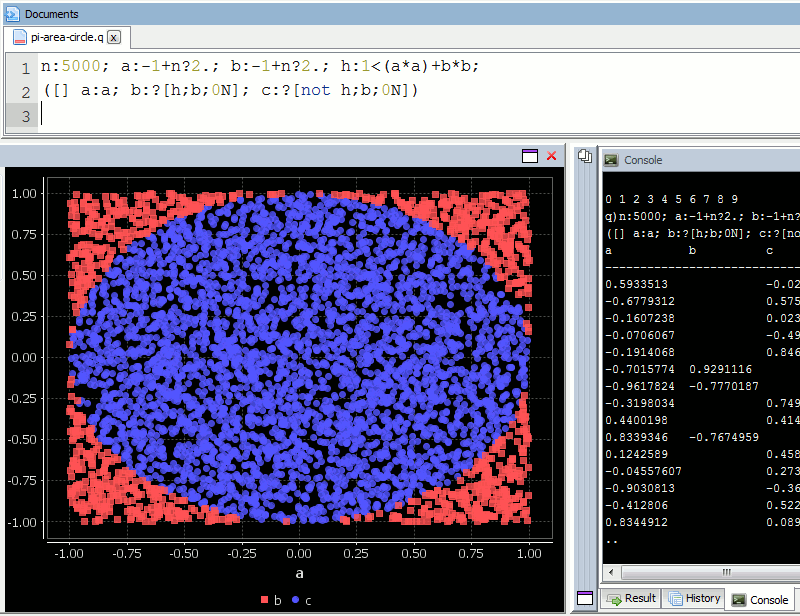
We know the area of our bounding square is 2*2 and that areaOfCircle=Pi*r*r, where r is 1. Therefore we can see that:
areaOfCircle = shadedRatio*areaOfSquare

Pi = shadedRatio * 4
q)4*sum[not h]%count h
3.141208
The wikipedia article on monte carlo method steps through this same example, as you can see their diagram looks similar:
December 10th, 2013 by Ryan Hamilton
In a previous post I looked at using the monte carlo method in kdb to find the outcome of rolling two dice. I also posed the question:
How many people do you need before the odds are good (greater than 50%) that at least two of them share a birthday?
In our kdb+ training courses I always advise breaking the problem down step by step, in this case:
- Consider making a function to examine the case where there are N people.
- Generate lists of N random numbers between 0-365 representing their birthdays.
- Find lists that contain collisions.
- Find the number of collisions per possibilities examined.
- Apply our function for finding the probability for N people to a list for many possibilities of N.
In kdb/q:
Plotting our data in using qStudio charting for kdb we get:
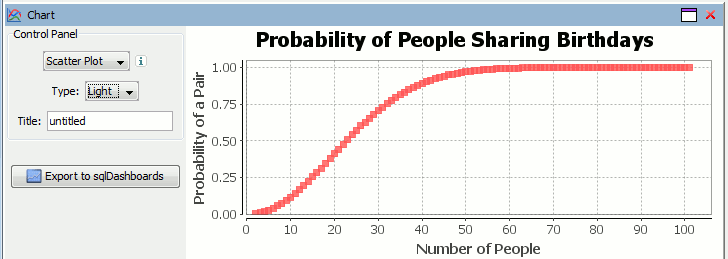
Therefore as you can see from either the q code or the graph, you need 23 people to ensure there’s a 50% chance that atleast 2 people in the room share a birthday. For more details see the wikipedia page. This still leaves us with the other problem of finding Pi using the monte carlo method in kdb.
December 3rd, 2013 by Ryan Hamilton
 Performing probability questions in kdb/q is simple. I recently got asked how to find the probability of rolling a sum of 12 with two dice. We’ll look at two approaches to finding the likely outcomes in kdb/q:
Method 1 – Enumeration of all possibilities
Step by step we:
- Generate the possible outcomes for one die.
- Generate all permutations for possible outcomes of two dice, find the sum of the dice.
- Count the number of times each sum occurs and divide by all possible outcomes to get each probability.
Method 2 – Monte Carlo Simulation
Alternatively , if it hadn’t occurred to us to use cross to generate all possible outcomes, or for situations where there may be too many to consider. We can use Monte Carlo method to simulate random outcomes and then similarly group and count their probability.
q)1+900000?/:6 6 / random pairs of dice rolls

2 5 6 6 2 4 3 1 5 1 1 4 6 5 3 4 2 4 1 2 3 6 6 1 1 3 6 3 6 2 3 1 5 4 4 4 6 3 1 3 1 2 5..

4 4 4 5 1 4 3 6 5 1 4 4 3 4 1 1 1 5 4 5 2 4 4 4 5 2 1 2 6 5 2 4 3 1 4 2 1 1 3 4 6 5 1..

q)/ same as before, count frequency of each result

q)(2+til 11)#{x%sum x} count each group sum each flip 1+900000?/:6 6

2 | 0.02766

3 | 0.05559

4 | 0.08347

5 | 0.11085

6 | 0.1391822

7 | 0.1669078

8 | 0.1386156

9 | 0.1112589

10| 0.08317222

11| 0.05556222

12| 0.02773111
Therefore the probability of rolling a sum of 12 with two dice is 1/36 or 0.27777. Here’s the similar dice permutation problem performed in java.
Kdb Problem Questions
If you want to try using the monte carlo method yourself try answering these questions:
- The Birthday Paradox: How many people do you need before the odds are good (greater than 50%) that at least two of them share a birthday?
- Finding the value of Pi. Consider a square at the origin of a coordinate system with a side of length 1. Now consider a quarter circle inside of the square, this circle has a radius of 1, therefore its area is pi/4. For a point (X,Y) to be inside of a circle of radius 1, its distance from the origin (X ², Y²) will be less than or equal to 1. We can generate random (X,Y) positions and determine whether each of them are inside of the circle. The ratio of those inside to outside will give the area. (bonus points for using multiple threads)
July 8th, 2013 by Ryan Hamilton
qStudio is an editor for kdb+ database by kx systems. Version 1.28 of qStudio is now available for download:
http://www.timestored.com/qstudio/
Changes in the latest version include:
- Added Csv Loader (pro)
- Added qUnit unit testing (pro)
- Bugfix to database management column copying.
- Export selection/table bugs fixed and launches excel (thanks Jeremy / Ken)
The Kdb+ Csv Loader allows loading local files onto a remote kdb+ server easily from within a GUI.
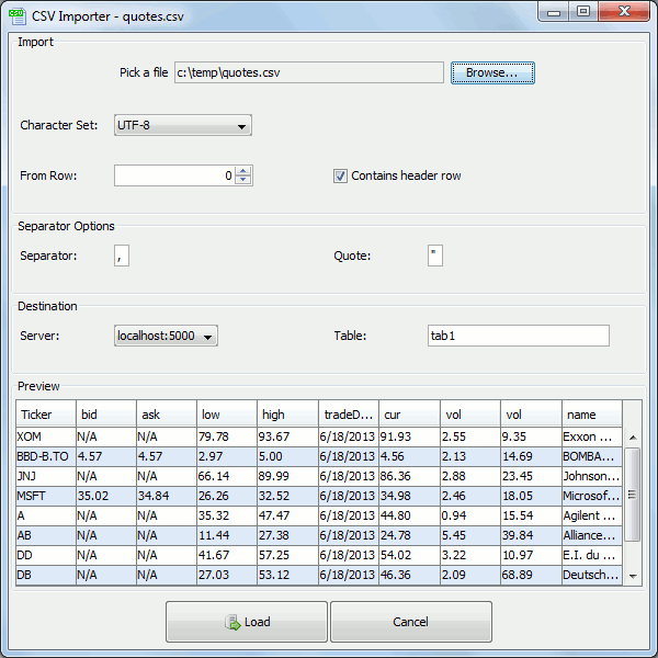
For step-by-step instructions see the qStudio loader help.
qUnit allows writing unit tests for q code in a format that will be familiar to all those who have used junit,cunit or a similar xunit based test framework. Tests depend on assertions and the results of a test run are shown as a table like so:
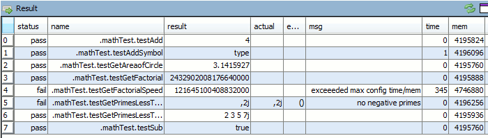
Tests are specified as functions that begin with the test** prefix and can have time or memory limits specified.
May 15th, 2013 by Ryan Hamilton
Sanket Agrawal just posted some very cool code to the k4 mailing list for finding the longest common sub-sequences. This actually solves a problem that some colleagues had where they wanted to combine two tickerplant feeds that never seemed to match up. Here’s an example:
q)/ assuming t is our perfect knowledge table
q)t
time sym size price
------------------------
09:00 A 8 7.343062
09:01 A 0 5.482385
09:02 B 5 8.847715
09:03 A 1 6.78881
09:04 B 5 3.432312
09:05 A 0 0.2801381
09:06 A 2 3.775222
09:07 B 3 1.676582
09:08 B 7 7.163578
09:09 B 4 3.300548
Let us now create two tables, u and v, neither of which contain all the data.
q)u:t except t 7 8

q)v:t except t 1 2 3 4

q)u

time sym size price

------------------------

09:00 A 8 7.343062

09:01 A 0 5.482385

09:02 B 5 8.847715

09:03 A 1 6.78881

09:04 B 5 3.432312

09:05 A 0 0.2801381

09:06 A 2 3.775222

09:09 B 4 3.300548

q)v

time sym size price

------------------------

09:00 A 8 7.343062

09:05 A 0 0.2801381

09:06 A 2 3.775222

09:07 B 3 1.676582

09:08 B 7 7.163578

09:09 B 4 3.300548
We can find the indices that differ using Sankets difftables function
q)p:diffTables[u;v;t `sym;`price`size]

q)show p 0; / rows in u that are not in v

1 2 3 4

q)show p 1; / rows in v that are not in u

3 4
/ combine together again
q)`time xasc (update src:`u from u),update src:`v from v p 1
time sym size price src
----------------------------
09:00 A 8 7.343062 u
09:01 A 0 5.482385 u
09:02 B 5 8.847715 u
09:03 A 1 6.78881 u
09:04 B 5 3.432312 u
09:05 A 0 0.2801381 u
09:06 A 2 3.775222 u
09:07 B 3 1.676582 v
09:08 B 7 7.163578 v
09:09 B 4 3.300548 u
q)t~`time xasc u,v p 1
1b
The code can be downloaded at:
http://code.kx.com/wsvn/code/contrib/sagrawal/lcs/miller.q
http://code.kx.com/wsvn/code/contrib/sagrawal/lcs/myers.q
Thanks Sanket.
Algorithm details:
Myers O(ND): http://www.xmailserver.org/diff2.pdf
Miller O(NP): http://www.bookoff.co.jp/files/ir_pr/6c/np_diff.pdf