Archive for the 'kdb+' Category
February 27th, 2017 by Ryan Hamilton
qUnit has added a new HTML report to allow visually easily seeing the difference between expected kdb results and actual results. To generate a report you could call:
.qunit.generateReport[.qunit.runTests[]; `:html/qunit.html]
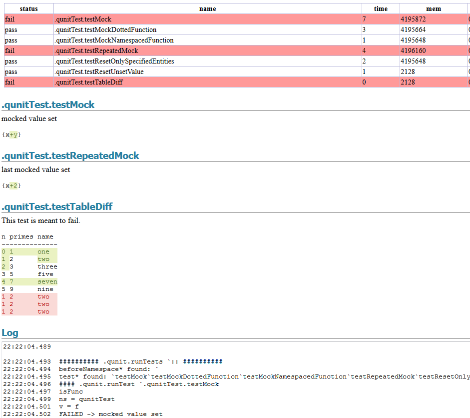
It’s also added a
.qunit.assertKnown[actualResult; expectedFilename; msg]
call to allow comparing an actual results to a file on disk. While allow easy updating of that file and avoiding naming collisions.
February 7th, 2017 by admin
This post is a walkthrough of my implementation in Q of the RosettaCode task ‘Death Star’.
The code is organized as general-purpose bitmap generator which can be used in other projects, and a client specific to the task of deathstar-drawing. The interface is a function which passes a map of pixel position to pixel value. The map can be a mapping function, or alternatively a 2D array of pixel values. The bitmap generator raster-scans the image, getting pixel values from either a mapping function or a mapped array.
genheader follows directly from the referenced BMP Wikipedia article.
genbitmap and genrow perform a raster scan of the image to be constructed. genbitmap steps along the vertical axis, calling genrow, which steps along the pixels of the current line, in turn calling fcn, the pixel-mapping function passed in by the client.
A sample client is included in comments, the simplest possible demonstration of shape and color (a circular mask selecting between two fill colors):
Conveniently, functions and arrays can be equivalently accessed in Q.
Here is an array-passing client which replicates the first example in the Wikipedia article on BMP format.
Element ordering can be confusing at first glance: Byte order for RGB pixels is B,G,R. Also, rows are indexed from bottom to top, and since bitmaps are in row-major order, the first and second array indices designated x and y correspond to the y and x image axes respectively.

After centering the image fcn applies several masks:
is calculates the orientation of a point on a sphere, and then a pixel value for that point, using the dot product of l, the light source direction, and s, the surface orientation. A correction of (1+value)/2 is applied, to achieve the ‘soft’ appearance of a space object in a movie. Alternatively we might have suppressed negative illumination values, to get the high-contrast appearance of an actual space object.
We might want to generate images of the death star at different rotations, however due to some simplifying assumptions we can’t rotate the weapon face to the side without glitching. We calculate z1 and z2 to select between the forward surface of the death star and the rearward surface of the weapon face. We should also calculate z3, the forward surface of the weapon face sphere, and z4, the rearward surface of the death star:
z3:170+z[x2;y;r];
z4:-z1;
Then the masks can be modified so that when z3 > z1 > z4 > z2, an additional bit of background is visible through the carved-out chunk of the deathstar.
TODO: discuss limitations of mask-and-fill; alternative approaches; display-list; …
TODO: discuss animation; …
TODO: discuss three-component architecture: orchestrator, world, bitmap generator
TODO: … conclusions
June 25th, 2016 by Ryan Hamilton
qStudio 1.41 is now available to download.
It adds the ability to use custom Security Authentications and custom JDBC drivers.
By automatically loading .jar plugins from libs folder.
After a few users reported issues around “watched expressions” we are removing the ctrl+w shortcut as it was often getting used by mistake. The last change was some internal work to improved startup/shutdown logging for debugging purposes..
April 26th, 2016 by Ryan Hamilton

Recently there was a post on SQL tips by the JOOQ guys. I love their work but I think standard SQL is not the solution to many of these problems. What we need is something new or in this case old, that is built for such queries. What do I mean, well let’s look through their examples reimplemented in qsql and I’ll show you how much shorter and simpler this could be.
Everything is a table
In kdb we take this a step further and make tables standard variables, no special notation/treatment, it’s a variable like any other variable in your programming language. Instead of messing about with value()() we define a concise notation to define our variables like so:
Data Generation with Recursive SQL
This is the example syntax they have used to define two tables and then join them:
What to hell! If I want variables, let’s have proper variables NOT “Common Table Expressions”.
I created two tables a and b then I joined them sideways. See how simple that was.
Running Total Calculations
Oh dear SQL how badly you have chosen your examples. Running calculations are to APL/qSQL as singing is to Tom Jones, we do it everyday all day and we like it. In fact the example doesn’t even give the full code. See this SO post for how these things get implemented. e.g. Standard SQL Running Sum
qSQL table Definition and Running Sum:
Finding the Length of a Series
This is their code:
This is KDB:
In 1974 Ken Iverson gave a talk on APL. He described how he reduced it down to a core set of operations that everything could be made from. Using these simple building blocks you could make some really cool things. It’s sad to think we may not have came that far.
qSQL/kdb is a database based on the concept of ordered lists, carrying over many ideas from APL that make array operations shorter and simpler. If you like what you see we provide tutorials on kdb to get started, this intro is a good place to get started.
We also have free online kdb training for students.
February 24th, 2016 by admin
First, in case you haven’t heard about it kdb has a standard SQL mode, you can send queries prefixed with s) and they will be interpreted as standard SQL like so:
Notice how the standard “and” syntax worked when I used s) but without it, q’s right to left evaluation causes problems. It’s about now that a lot of people get very excited, they think great I can skip learning that q-sql and use my standard SQL. Sometimes the look of joy on their faces transforms to frustration once they start using it. So let’s look at what works:
| Operation |
Works? |
| Standard SQL Inserts |
Yes |
| ORDER BY |
half works |
| COUNT |
Yes |
| DELETE |
Yes |
| UPDATE |
Yes |
| String matching |
slightly works |
| NOT |
NO |
| IN |
Yes |
| GROUP BY |
Yes |
| LIMIT / TOP |
NO |
| Date Times |
NO |
Standard SQL Inserts work
ORDER BY half works
“ORDER BY” will sort the columns in ascending order, attempting to use DESC has no effect.
COUNT works
DELETE works
UPDATE works
String matching slightly works
NOT fails
Modifying our String query slightly by adding NOT throws an error. My guess is that the interpreter has got confused.
IN works
GROUP BY works
LIMIT / TOP does not work
Date Times Don’t Work Right
Overall standard SQL support in kdb has got much better. However I would still recommend only using the s) syntax for plugging into an existing jdbc/odbc visualization tool and getting some immediate simple results. For any form of complex queries on strings, joins etc. support is either not there or the result may not be what you expect.
February 15th, 2016 by admin
qStudio 1.40 is now available to download.
The latest changes include:
- No need to save changes before shutdown, unsaved changes stored till reopened.
- Add sqlchart to system path.
- Fix display of tables with underscore in the name.
- Database documenter/report enhancements
- Improved code printing
- FileTreePanel much more efficient at displaying large number of files.
November 5th, 2015 by John Dempster
Previously on our blog we had a lively debate about a possibly Open Sourced kdb+ , unfortunately kx now seems to be moving the opposite direction. In a recent announcement they are now restricting “32-bit kdb+ for non-commercial use only”. The timing is particularly unfortunate as:
Alternative (far less enterprise proven) solutions are available:
- MAN AHL have released Arctic an open source Market Data platform based on python and MongoDB
- Kerf Database – A DB aimed at the same market as kdb has now partnered with Briarcliff-Hall and is making greater sales inroads
This renewed interest in kdb alternatives hasn’t so far delivered a kdb+ killer but I fear in time it will.
May 2nd, 2015 by admin
An intellij keyword file is now available to provide syntax highlighting of kdb code in intellij:
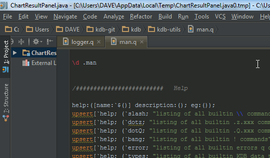
q Code Intellij Highlighting
To install it copy this xml file to this directory:
C:\Users\USERNAME\.IdeaIC14\config\filetypes
Where USERNAME is obviously your username. Then restart intellij and open a .q file.
We’ve updated our notepad++ qlang.xml to provide code folding and highlighting of the .Q/.z namespaces.
May 2nd, 2015 by admin
We’ve now posted all source code from this website on our github kdb page.
Additionally we are open sourcing qunit, our kdb testing framework.
We look forward to receiving pull requests to fix our (hopefully few) bugs.
April 23rd, 2015 by admin
Since our last qStudio kdb+ IDE announcment we have added a lot of new features:
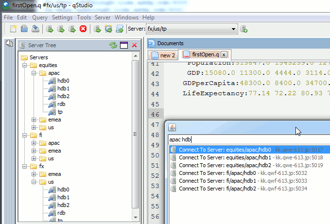
Bulk importing kdb server lists
There’s a lot of new features to allow supporting a huge number of servers efficiently:
- Support importing HUGE number of servers:
- 5000+ server connections are now supported
- To prevent massive memory use, the object tree for a server is no longer refreshed at startup only on connection.
- Allow specifying default username/password once for all servers
- Allow nested connection folders
- Add critical color option – servers with prod in name get highlighted in red
- Sort File Tree Alphabetically
- Numerous bugfixes including:
- Fix critical Mac bug that prevented launching in some instances
- Fix query cancelling