Archive for the 'kdb+' Category
October 20th, 2014 by admin
Based on user requests we have released a number of new features with qStudio 1.36:
Download the latest ->qStudio<- now.
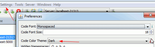
Dark Code Editor Themes
Which can be set under settings->preferences
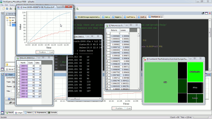
Open Results and Charts in New Window
To expand a panel into a new window click the “pop-out” icon.
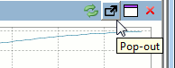
This will bring up the result in a new window:
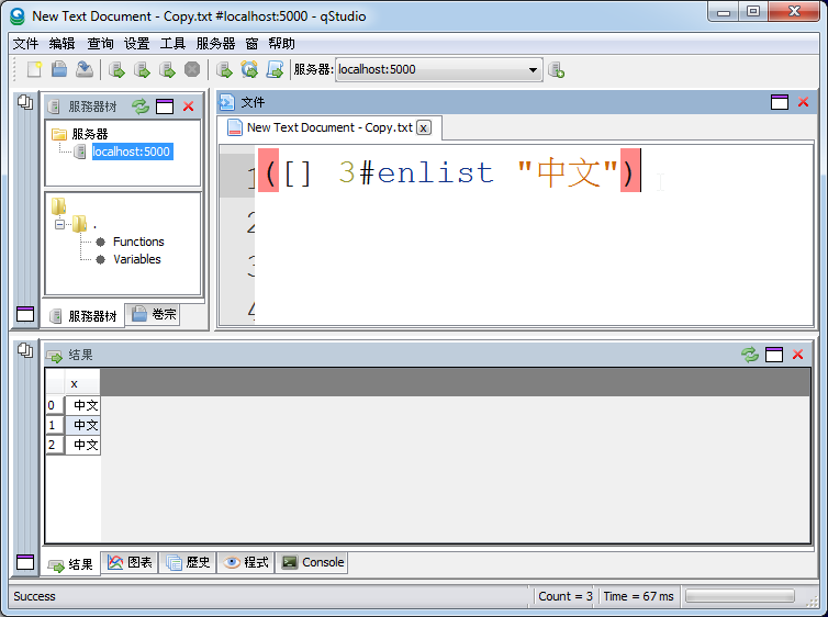
UTF-8 Chinese Language Support
October 8th, 2014 by admin
kdb+ London Contract – £800 p/day
kdb+ belfast Citigroup Contract £400 p/day
Java Poland £150 p/day

September 8th, 2014 by admin
sqlDashboards are included as a bundle with qStudio, part of that package is a command line utility called sqlChart that allows generating customized sql charts from the command line.
Checkout the video to see how you can create a chart based on data from a kdb+ database in 2 minutes:
The sqlChart page has all the documentation you need, Download the qstudio.zip to try it now.
The q Code
Help Screen
April 10th, 2014 by admin
Kdb does not have built-in functions for bitwise and,or,xor operations, we are going to create a C DLL extension that provides bitwise operators.
To download the source and definitions for and/or/xor bitwise operations click here
If your new to extending Kdb+ see this tutorial on writing a DLL for Kdb+
I also thought this would be a good opportunity to look at using q-code to generate C code, to generate Kdb Dll’s. When converting an existing library to work with Kdb or writing similar functions for different types, there’s a lot of repetitive coding. Either you can use macros or you can use one language to generate another, to save a lot of typing. Let’s look at bitwise operations as an example of what I mean:
If I wanted to write a bitwise and function band that takes two lists and performs a corresponding operation, we could write the C functions like so:
Notice the similarity between the bandJJ and bandII functions. Plus if we want to handle the case where the second argument is an atom we need an entire other set of C functions similar to bandJ to handle that. This is soon beginning to spiral beyond an easy copy paste job. Instead I used the following 20 lines of q code to generate the 130 lines of C code:
This generates my C code, a .def file exporting the functions that I want to provide and creates a .q file that loads those functions into kdb. Which means any time I add a function or want to support a new type, everything is done for me. let’s look at our functions in action:
Yes the q code is messy (it could be improved) but the concept of dynamically generating your imports can be a real time saver.
This code is not intended for reliability or performance, use at your own risk! If however bitwise operations are a topic that interest you I recommend this article on: Writing a fast vectorised OR function for Kdb.
March 30th, 2014 by Ryan Hamilton
Often at the start of one of our training courses I’m asked why banks use the Kdb Database for their tick data.
- One well known reason is that kdb is really fast at typical financial time-series queries
(due to Kdbs column-oriented architecture).
- Another reason is that qSQL is extremely expressive and well suited for time-series queries.
To demonstrate this I’d like to look at three example queries, comparing qSQL to standard SQL.
SQL Queries dependent on order
From the table below we would like to find the price change between consecutive rows.
| time |
price |
| 07:00 |
0.9 |
| 08:30 |
1.5 |
| 09:59 |
1.9 |
| 10:00 |
2 |
| 12:00 |
9 |
|
|
q Code
In kdb qSQL this would be the extremely simple and readable code:
Standard SQL
In standard SQL there are a few methods, we can use. The simplest is if we already have a sequential id column present:
Even for this simple query our code is much longer and not as clear to read. If we hadn’t had the id column we would have needed much more code to create a temporary table with row numbers. As our queries get more complex the situation gets worse.
Select top N by category
Given a table of stock trade prices at various times today, find the top two trade prices for each ticker.
trade table
| time |
sym |
price |
| 09:00 |
a |
80 |
| 09:03 |
b |
10 |
| 09:05 |
c |
30 |
| 09:10 |
a |
85 |
| 09:20 |
a |
75 |
| 09:30 |
b |
13 |
| 09:40 |
b |
14 |
|
|
qSQL Code
In q code this would be select 2 sublist desc price by sym from trade, anyone that has used kdb for a few days could write the query and it almost reads like english. Select the prices in descending order by sym and from those lists take the first 2 items (sublist).
SQL Code
In standard SQL a query that depends on order is much more difficult , witness the numerous online posts with people having problems: stackoverflow top 10 by category, mysql first n rows by group, MS-SQL top N by group. The nicest solution, if your database supports it, is:
The SQL version is much harder to read and will require someone with more experience to be able to write it.
Joining Records on Nearest Time
Lastly we want to consider performing a time based join. A common finance query is to find the prevailing quote for a given set of trades. i.e. Given the following trade table t and quote table q shown below, we want to find the prevailing quote before or at the exact time of each trade.
trades t
| time |
sym |
price |
size |
| 07:00 |
a |
0.9 |
100 |
| 08:30 |
a |
1.5 |
700 |
| 09:59 |
a |
1.9 |
200 |
| 10:00 |
a |
2 |
400 |
| 12:00 |
b |
9 |
500 |
| 16:00 |
a |
10 |
800 |
|
quotes q
| time |
sym |
bid |
| 08:00 |
a |
1 |
| 09:00 |
b |
9 |
| 10:00 |
a |
2 |
| 11:00 |
b |
8 |
| 12:00 |
b |
8.5 |
| 13:00 |
a |
3 |
| 14:00 |
b |
7 |
| 15:00 |
a |
4 |
|
|
In qSQL this is: aj[`sym`time; t; q], which means perform an asof-join on t, looking up the nearest match from table q based on the sym and time column.
In standard SQL, again you’ll have difficulty: sql nearest date, sql closest date even just the closest lesser date isn’t elegant. One solution would be:
It’s worth pointing out this is one of the queries that is typically extremely slow (minutes) on row-oriented databases compared to column-oriented databases (at most a few seconds).
qSQL vs SQL
Looking at the simplicity of the qSQL code compared to the standard SQL code we can see how basing our database on ordered lists rather than set theory is much more suited to time-series data analysis. By being built from the ground up for ordered data and by providing special time-series based joins, kdb let’s us form these example queries using very simple expressions. Once we need to create more complex queries and nested selects, attempting to use standard SQL can quickly spiral into a verbose unmaintainable mess.
I won’t say qSQL can’t be cryptic 🙂 but for time-series queries qSQL will mostly be shorter and simpler than trying to use standard SQL.
If you think you have shorter SQL code that solves one of these examples or you are interested in one of our kdb training courses please get in touch.
March 30th, 2014 by Ryan Hamilton
In this tutorial we are going to recreate this example RSI calculation in q, the language of the kdb database.
The relative strength index (RSI) is a technical indicator used in the analysis of financial markets. It is intended to chart the current and historical strength or weakness of a stock or market based on the closing prices of a recent trading period. The RSI is classified as a momentum oscillator, measuring the velocity and magnitude of directional price movements. Momentum is the rate of the rise or fall in price.
The RSI computes momentum as the ratio of higher closes to lower closes: stocks which have had more or stronger positive changes have a higher RSI than stocks which have had more or stronger negative changes. The RSI is most typically used on a 14 day timeframe, measured on a scale from 0 to 100, with high and low levels marked at 70 and 30, respectively. Shorter or longer timeframes are used for alternately shorter or longer outlooks. More extreme high and low levels—80 and 20, or 90 and 10—occur less frequently but indicate stronger momentum.
.
Stock Price Time-Series Data
We are going to use the following example data, you can download the csv here or the excel version here.
| Date |
QQQQ Close |
Change |
Gain |
Loss |
Avg Gain |
Avg Loss |
RS |
14-day RSI |
| 2009-12-14 |
44.34 |
|
|
|
|
|
|
|
| 2009-12-15 |
44.09 |
-0.25 |
0.00 |
0.25 |
|
|
|
|
| 2009-12-16 |
44.15 |
0.06 |
0.06 |
0.00 |
|
|
|
|
| 2009-12-17 |
43.61 |
-0.54 |
0.00 |
0.54 |
|
|
|
|
| 2009-12-18 |
44.33 |
0.72 |
0.72 |
0.00 |
|
|
|
|
| 2009-12-21 |
44.83 |
0.50 |
0.50 |
0.00 |
|
|
|
|
| 2009-12-22 |
45.10 |
0.27 |
0.27 |
0.00 |
|
|
|
|
| 2009-12-23 |
45.42 |
0.33 |
0.33 |
0.00 |
|
|
|
|
| 2009-12-24 |
45.84 |
0.42 |
0.42 |
0.00 |
|
|
|
|
| 2009-12-28 |
46.08 |
0.24 |
0.24 |
0.00 |
|
|
|
|
| 2009-12-29 |
45.89 |
-0.19 |
0.00 |
0.19 |
|
|
|
|
| 2009-12-30 |
46.03 |
0.14 |
0.14 |
0.00 |
|
|
|
|
| 2009-12-31 |
45.61 |
-0.42 |
0.00 |
0.42 |
|
|
|
|
| 2010-01-04 |
46.28 |
0.67 |
0.67 |
0.00 |
|
|
RS |
RSI |
| 2010-01-05 |
46.28 |
0.00 |
0.00 |
0.00 |
0.24 |
0.10 |
2.39 |
70.53 |
| 2010-01-06 |
46.00 |
-0.28 |
0.00 |
0.28 |
0.22 |
0.11 |
1.97 |
66.32 |
| 2010-01-07 |
46.03 |
0.03 |
0.03 |
0.00 |
0.21 |
0.10 |
1.99 |
66.55 |
| 2010-01-08 |
46.41 |
0.38 |
0.38 |
0.00 |
0.22 |
0.10 |
2.27 |
69.41 |
| 2010-01-11 |
46.22 |
-0.19 |
0.00 |
0.19 |
0.20 |
0.10 |
1.97 |
66.36 |
| 2010-01-12 |
45.64 |
-0.58 |
0.00 |
0.58 |
0.19 |
0.14 |
1.38 |
57.97 |
| 2010-01-13 |
46.21 |
0.57 |
0.57 |
0.00 |
0.22 |
0.13 |
1.70 |
62.93 |
| 2010-01-14 |
46.25 |
0.04 |
0.04 |
0.00 |
0.20 |
0.12 |
1.72 |
63.26 |
| 2010-01-15 |
45.71 |
-0.54 |
0.00 |
0.54 |
0.19 |
0.15 |
1.28 |
56.06 |
| 2010-01-19 |
46.45 |
0.74 |
0.74 |
0.00 |
0.23 |
0.14 |
1.66 |
62.38 |
| 2010-01-20 |
45.78 |
-0.67 |
0.00 |
0.67 |
0.21 |
0.18 |
1.21 |
54.71 |
| 2010-01-21 |
45.35 |
-0.43 |
0.00 |
0.43 |
0.20 |
0.19 |
1.02 |
50.42 |
| 2010-01-22 |
44.03 |
-1.33 |
0.00 |
1.33 |
0.18 |
0.27 |
0.67 |
39.99 |
| 2010-01-25 |
44.18 |
0.15 |
0.15 |
0.00 |
0.18 |
0.26 |
0.71 |
41.46 |
| 2010-01-26 |
44.22 |
0.04 |
0.04 |
0.00 |
0.17 |
0.24 |
0.72 |
41.87 |
| 2010-01-27 |
44.57 |
0.35 |
0.35 |
0.00 |
0.18 |
0.22 |
0.83 |
45.46 |
| 2010-01-28 |
43.42 |
-1.15 |
0.00 |
1.15 |
0.17 |
0.29 |
0.59 |
37.30 |
| 2010-01-29 |
42.66 |
-0.76 |
0.00 |
0.76 |
0.16 |
0.32 |
0.49 |
33.08 |
| 2010-02-01 |
43.13 |
0.47 |
0.47 |
0.00 |
0.18 |
0.30 |
0.61 |
37.77 |
RSI Formulas
The formulas behind the calculations used in the table are:
- First Average Gain = Sum of Gains over the past 14 periods / 14.
- First Average Loss = Sum of Losses over the past 14 periods / 14
All subsequent gains than the first use the following:
- Average Gain = [(previous Average Gain) x 13 + current Gain] / 14.
- Average Loss = [(previous Average Loss) x 13 + current Loss] / 14.
- RS = Average Gain / Average Loss
- RSI = 100 – 100/(1+RS)
Writing the Analytic in q
We can load our data (rsi.csv) in then apply updates at each step to recreate the table above:
Code kindly donated by Terry Lynch
Rather than create all the intermediate columns we can create a calcRsi function like so:
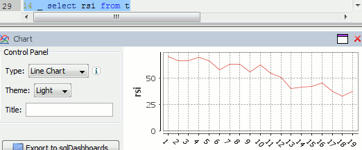
Finally we can visualize our data using the charting functionality of qStudio (an IDE for kdb):
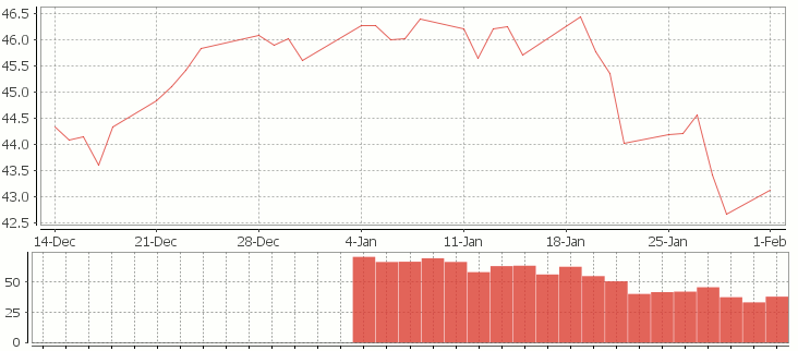
RSI Relative Strength Index stock chart for QQQQ created using qStudio
Or to plot RSI by itself (similar to original article
Writing kdb analytics such as Relative Strength Index is covered in our kdb training course, we offer both public kdb training courses in New York, London, Asia and on-site kdb courses at your offices, tailored to your needs.
March 30th, 2014 by admin
While doing the project euler programming challenges it annoyed me how verbose the java answers would have to be compared to kdb. Then I got to wondering if I could create functions like til,mod,where,asc etc. in java and use them to create really short answers. Once I had the basic functions working, I wondered if I could get a working q) prompt…
I ended up with a prompt that let me run the following valid q code within the java runtime:
where[or[ =[0; mod[til[1000];3]]; =[0; mod[til[1000];5]] ]]
Download the jkdb functional kdb code
The Code
How it Works
My Jkdb class has a number of statically defined functions that accept arrays of ints/doubles and return arrays/atoms of int/double. An example is asc:
In the background each line you type has the square brackets and semi-colons converted to () and comma which are now valid java function calls. The amended string gets added to a .java file, compiled, ran and the output shown each time you press enter. Since I statically imported my class that has the til(x),max(x) etc functions, the code is valid java and works. This is why we can only use functional[x;y] form calls and not the infix notation x func y as I didn’t want to write a parser.
Interesting Points that would occur in Kdb
- All of the functions usually accept int,double, int[],double[] and boolean[] as their arguments and the various combinations. It is annoying having to copy paste these various combinations, I assume in kdb they use C macros to generate the functions, we could do something similar by writing java code to write the java functions.
- The functions I wrote often modify the array passed in, this gives us insight to why in the kdb C api you have to reference count properly, when the reference is 0 the structure is probably reused.
What use is this?
Almost entirely useless 🙂 I use the java class to occasionally spit out some sample data for tests I write. It was however insightful to get an idea of how kdb works under the covers. If you found this interesting you might also like kona an open source implementation of kdb.
I’d be interested in hearing:
- Have you tried kona? Did it work well?
- Have you found a functional library that gives you similar expressiveness to kdb for java?
- Tried Scala? Clojure?
The Jkdb provided functions are:
| til where |
| equal= |
| index@ |
| choose(x,y) ? – only supports x and y as int’s to choose random numbers |
|
| or(x,y) and(x,y) |
| mul(x,y) add(x,y) |
| mod(x,y) |
|
| floor ceiling abs |
| cos sin tan |
| acos asin atan |
| sqrt |
|
| asc desc max min reverse |
| sum sums prd prds |
|
| set(String key, Object value) |
| get(String key) |
March 29th, 2014 by Ryan Hamilton
Let’s look at how to write moving average analytics in q for the kdb database. As example data (mcd.csv) we are going to use stock price data for McDonalds MCD. The below code will download historical stock data for MCD and place it into table t:
Simple Moving Average
The simple moving average can be used to smooth out fluctuating data to identify overall trends and cycles. The simple moving average is the mean of the data points and weights every value in the calculation equally. For example to find the moving average price of a stock for the past ten days, we simply add the daily price for those ten days and divide by ten. This window of size ten days then moves across the dates, using the values within the window to find the average. Here’s the code in kdb for 10/20 day moving average and the resultant chart.
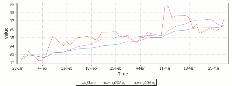
Simple Moving Average Stock Chart Kdb (Produced using qStudio)
What Exponential Moving Average is and how to calculate it
One of the issues with the simple moving average is that it gives every day an equal weighting. For many purposes it makes more sense to give the more recent days a higher weighting, one method of doing this is by using the Exponential Moving Average. This uses an exponentially decreasing weight for dates further in the past.The simplest form of exponential smoothing is given by the formula:

where α is the smoothing factor, and 0 < α < 1. In other words, the smoothed statistic st is a simple weighted average of the previous observation xt-1 and the previous smoothed statistic st−1.
This table displays how the various weights/EMAs are calculated given the values 1,2,3,4,8,10,20 and a smoothing factor of 0.7: (excel spreadsheet)
| Values |
EMA |
|
Power |
Weight |
Power*Weight |
|
EMA (text using previous value) |
| 1 |
1 |
|
6 |
0.0005103 |
0.0005103 |
|
1 |
| 2 |
1.7 |
|
5 |
0.001701 |
0.003402 |
|
(0.7*2)+(0.3*1) |
| 3 |
2.61 |
|
4 |
0.00567 |
0.01701 |
|
(0.7*3)+(0.3*1.7) |
| 4 |
3.583 |
|
3 |
0.0189 |
0.0756 |
|
(0.7*4)+(0.3*2.61) |
| 8 |
6.6749 |
|
2 |
0.063 |
0.504 |
|
(0.7*8)+(0.3*3.583) |
| 10 |
9.00247 |
|
1 |
0.21 |
2.1 |
|
(0.7*10)+(0.3*6.6749) |
| 20 |
16.700741 |
|
0 |
0.7 |
14 |
|
(0.7*20)+(0.3*9.00247) |
To perform this calculation in kdb we can do the following:
(This code was originally posted to the google mail list by Attila, the full discussion can be found here)
This backslash adverb works as
The alternate syntax generalizes to functions of 3 or more arguments where the first argument is used as the initial value and the arguments are corresponding elements from the lists:
Exponential Moving Average Chart
Finally we take our formula and apply it to our stock pricing data, allowing us to see the exponential moving average for two different smoothing factors:
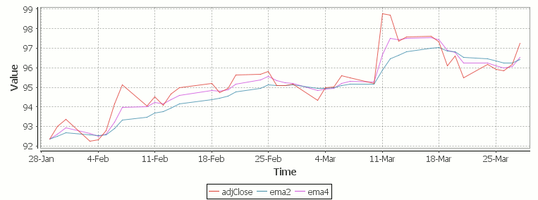
Exponential Moving Average Stock Price Chart produced using qStudio
As you can see with EMA we can prioritize more recent values using a chosen smoothing factor to decide the balance between recent and historical data.
Writing kdb analytics such as Exponential Moving Average is covered in our kdb training course, we regularly provide training courses in London, New York, Asia or our online kdb course is available to start right now.
March 4th, 2014 by John Dempster
qStudio is an IDE for kdb+, you can download it now.
The latest 1.31 release introduces a number of nice interface additions as requested by users:
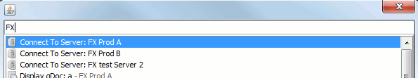
Command Palette
Quick change server -> Hit Ctrl+P to try the new Command Palette
It lets you run common qStudio actions by fuzzy matching on keywords:
Jump to Definition
Hit Ctrl+U Ctrl+I to get an outline of the current file.
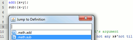
Or press Ctrl+D on a function call to jump to where it is defined.
Added User Preferences
Users had mentioned a number of connection and interface issues they wanted to be able to customize, these have been added:
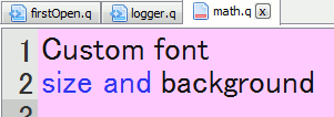
– Customize the editor font and it’s background color (per server setting, useful for red warning color when connected to prod machines)
– keep same connection open for every query
– Wrap every query with selected text before and after
Eval Line by Line
Do you ever query a line, move down, query next line, move down ….
Well try control+shift+enter within the code editor.
It evaluates the current line, returns it’s value and shifts to the next line.
e.g. for the code:
a:11
b:a*rand[10]
c:b*a
The console would show:
q)a:11
11
q)b:a*rand[10]
55
q)c:b*a
605
The qStudio help guide contains more details of all functionality.
December 15th, 2013 by Ryan Hamilton
In a previous post I looked at using the monte carlo method in kdb to find the outcome of rolling two dice. I also posed the question:
How can we find the value of Pi using the Monte Carlo method?
If we randomly chose an (x,y) location, we could calculate the distance of that points location ( sqrt[x²+y²] ) from the origin, this would tell us if that point lay within a circle or outside a circle, by whether the length was greater than our radius. The ratio of the points that fall within the circle relative to the square that bounds our circle, gives us the ratio of the areas.
A diagram is probably the easiest way to visualize this problem. If we generate two lists of random numbers between -1 to 1. And use those as the coordinates (x,y), then create a scatter plot that plots (x,y) in one colour where x²+y² is greater than 1 and a different colour where it is less than 1, we would find a pattern emerging…in qStudio it looks like this:
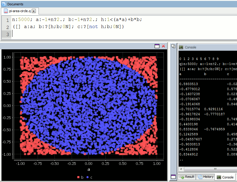
We know the area of our bounding square is 2*2 and that areaOfCircle=Pi*r*r, where r is 1. Therefore we can see that:
areaOfCircle = shadedRatio*areaOfSquare

Pi = shadedRatio * 4
q)4*sum[not h]%count h
3.141208
The wikipedia article on monte carlo method steps through this same example, as you can see their diagram looks similar: