Archive for the 'qStudio' Category
April 2nd, 2018 by admin
qStudio has added support for stacked bar charts:
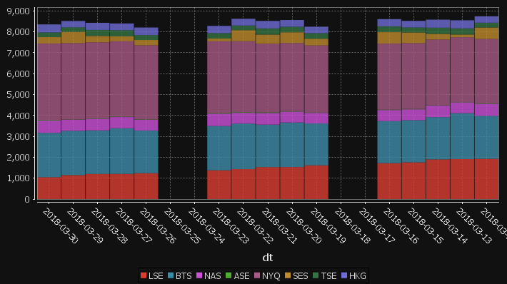
The chart format for this is: The first string columns are used as category labels. Whatever numeric columns appear next are a separate series in the chart. Each row in the data becomes one stacked bar. The table for the data shown above for example is:
| dt |
LSE |
BTS |
NAS |
ASE |
NYQ |
SES |
TSE |
HKG |
| 2018-03-30 |
1047 |
2120 |
592 |
25 |
3660 |
303 |
225 |
383 |
| 2018-03-29 |
1148 |
2118 |
528 |
10 |
3656 |
541 |
215 |
303 |
| 2018-03-28 |
1201 |
2085 |
555 |
17 |
3644 |
302 |
290 |
339 |
| 2018-03-27 |
1206 |
2182 |
535 |
21 |
3604 |
235 |
299 |
319 |
| 2018-03-26 |
1239 |
2041 |
515 |
16 |
3549 |
251 |
234 |
363 |
| 2018-03-25 |
0 |
0 |
0 |
0 |
0 |
0 |
0 |
0 |
| 2018-03-24 |
0 |
0 |
0 |
0 |
0 |
0 |
0 |
0 |
| 2018-03-23 |
1379 |
2115 |
595 |
29 |
3430 |
138 |
251 |
348 |
| 2018-03-22 |
1431 |
2179 |
517 |
25 |
3399 |
531 |
222 |
320 |
| 2018-03-21 |
1530 |
2032 |
558 |
29 |
3282 |
438 |
296 |
359 |
| 2018-03-20 |
1531 |
2134 |
520 |
23 |
3256 |
515 |
265 |
322 |
You may need to “kdb pivot” your original data to get it in the correct shape.
April 1st, 2018 by Ryan Hamilton
“The Financial Information eXchange (FIX) protocol is an electronic communications protocol initiated in 1992 for international real-time exchange of information related to the securities transactions and markets.”. You can see an example of a FIX message being parsed here.
What we care about is that an order goes through a lifecycle. From newly created to filled or removed. Anything that involves state-transitions or a lifecycle can be visualized as a graph. A graph depicts transitions from one state to another. Often SQL tables record every transition of that state. This can then be summarised into a count of the last state, giving something like the following:
| From |
To |
label |
cnt |
| PendingCancel |
Calculated |
Rejected |
50 |
| PendingReplace |
Calculated |
Rejected |
10 |
| PendingReplace |
Calculated |
Replaced |
40 |
| Calculated |
PendingReplace |
PendingReplace |
50 |
| Calculated |
Filled |
Trade |
9400 |
| Calculated |
Calculated |
Trade |
5239 |
| PendingCancel |
Removed |
Cancelled |
150 |
| Calculated |
PendingCancel |
PendingCancel |
200 |
| New |
Calculated |
Calculated |
9660 |
| New |
Removed |
Rejected |
140 |
| Created |
Removed |
Rejected |
300 |
| Created |
New |
New |
9800 |
qStudio now automatically converts this result table to DOT format and if you have graphviz“>graphviz installed and on the PATH, will generate the following:
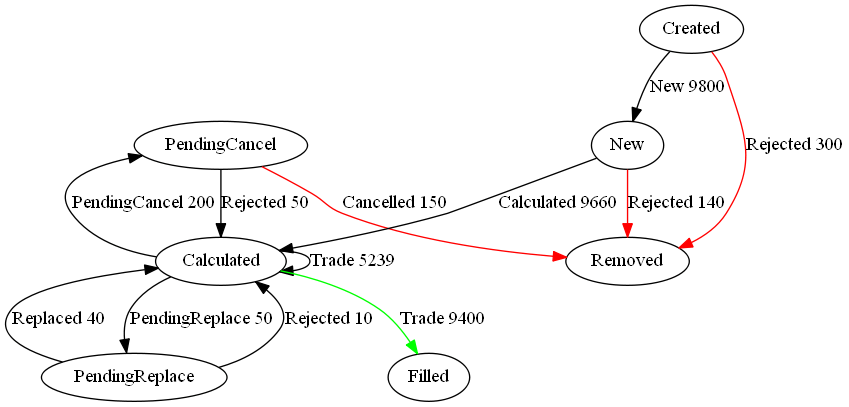
Note I did tweak the table a little to add styling like so:
update style:(`Filled`Removed!("color=green";"color=red")) To,label:(label,'" ",/:cnt) from currentFixStatus
The format is detailed again in our qStudio Chart Data Format page.
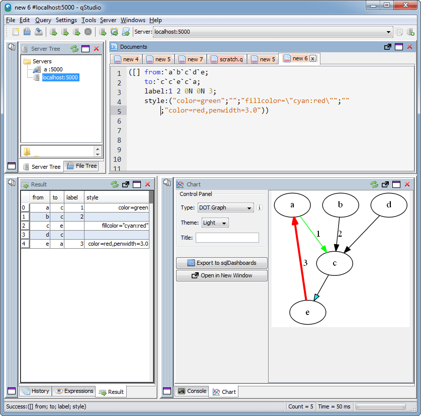
This is another even simpler example:
April 13th, 2017 by Ryan Hamilton
qStudio 1.43 Released. This:
- Adds stack traces to kdb 3.5+
- Fixes the mac bug where the filename wasn’t shown when trying to save a file.
- Fixes a number of multi-threading UI problems
Download it now.
April 13th, 2017 by Ryan Hamilton
kdb+ 3.5 had a significant number of changes:
- Debugger – At long last we can finally get stack traces when errors occur.
- Concurrent Memory Allocator – Supposedly better performance when returning large results from peach
- Port Reuse – Allow multiple processes to listen on same port. Assuming Linux Support
- Improved Performance – of Sorting and Searching
- Additional ujf function – Similar to uj from v2.x fills from left hand side
kdb Debugger
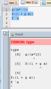
The feature that most interests us right now is the Debugging functionality. If you are not familiar with how basic errors, exceptions and stack movement is handled in kdb see our first article on kdb debugging here. In this short post we will only look at the new stack trace functionality.
Now when you run a function that causes an error at the terminal you will get the stack trace. Here’s a simple example where the function f fails:
Whatever depth the error occurs at we get the full depth stack trace, showing every function that was called to get there using .Q.bt[]:
The good news is that this same functionality is availabe in qStudio 1.43. Give it a try: qStudio.
Note: the ability to show stack traces relies on qStudio wrapping every query you send to the server with its own code to perform some analysis and return those values. By default wrapping is on as seen in preferences. If you are accessing a kdb server ran by someone else you may have to turn wrapping off as that server may limit which queries are allowed. Unfortunately stack tracing those queries won’t be easily possible.
That’s just the basics, there are other new exposed functions and variables, such as .Q.trp – for trapping calls and accessing traces that we are going to look at in more detail in future.
June 25th, 2016 by Ryan Hamilton
qStudio 1.41 is now available to download.
It adds the ability to use custom Security Authentications and custom JDBC drivers.
By automatically loading .jar plugins from libs folder.
After a few users reported issues around “watched expressions” we are removing the ctrl+w shortcut as it was often getting used by mistake. The last change was some internal work to improved startup/shutdown logging for debugging purposes..
February 15th, 2016 by admin
qStudio 1.40 is now available to download.
The latest changes include:
- No need to save changes before shutdown, unsaved changes stored till reopened.
- Add sqlchart to system path.
- Fix display of tables with underscore in the name.
- Database documenter/report enhancements
- Improved code printing
- FileTreePanel much more efficient at displaying large number of files.
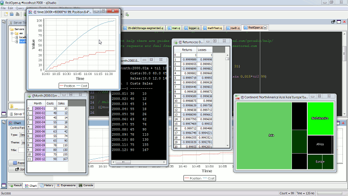
April 23rd, 2015 by admin
Since our last qStudio kdb+ IDE announcment we have added a lot of new features:
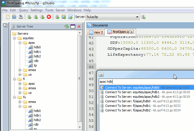
Bulk importing kdb server lists
There’s a lot of new features to allow supporting a huge number of servers efficiently:
- Support importing HUGE number of servers:
- 5000+ server connections are now supported
- To prevent massive memory use, the object tree for a server is no longer refreshed at startup only on connection.
- Allow specifying default username/password once for all servers
- Allow nested connection folders
- Add critical color option – servers with prod in name get highlighted in red
- Sort File Tree Alphabetically
- Numerous bugfixes including:
- Fix critical Mac bug that prevented launching in some instances
- Fix query cancelling
October 20th, 2014 by admin
Based on user requests we have released a number of new features with qStudio 1.36:
Download the latest ->qStudio<- now.
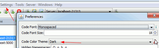
Dark Code Editor Themes
Which can be set under settings->preferences
Open Results and Charts in New Window
To expand a panel into a new window click the “pop-out” icon.
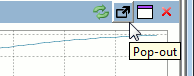
This will bring up the result in a new window:
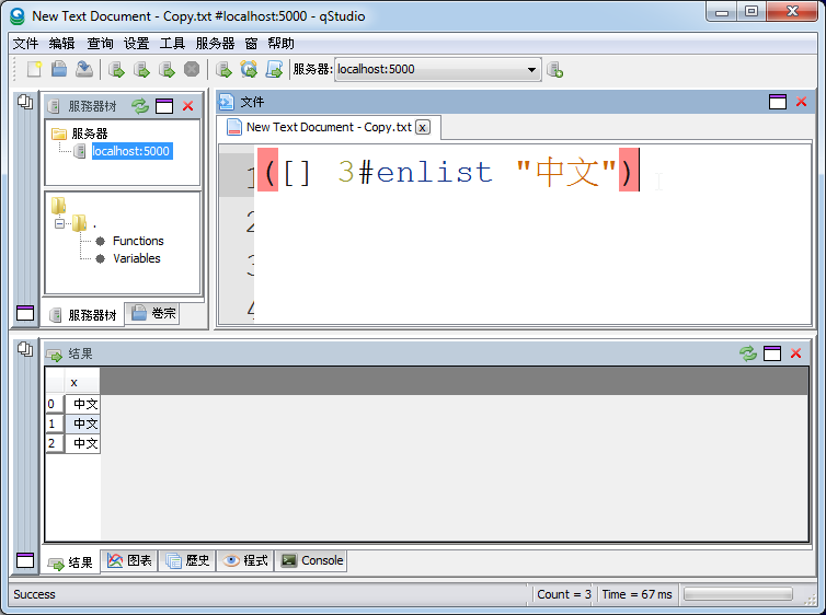
UTF-8 Chinese Language Support
September 8th, 2014 by admin
sqlDashboards are included as a bundle with qStudio, part of that package is a command line utility called sqlChart that allows generating customized sql charts from the command line.
Checkout the video to see how you can create a chart based on data from a kdb+ database in 2 minutes:
The sqlChart page has all the documentation you need, Download the qstudio.zip to try it now.
The q Code
Help Screen
March 30th, 2014 by Ryan Hamilton
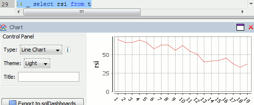
In this tutorial we are going to recreate this example RSI calculation in q, the language of the kdb database.
The relative strength index (RSI) is a technical indicator used in the analysis of financial markets. It is intended to chart the current and historical strength or weakness of a stock or market based on the closing prices of a recent trading period. The RSI is classified as a momentum oscillator, measuring the velocity and magnitude of directional price movements. Momentum is the rate of the rise or fall in price.
The RSI computes momentum as the ratio of higher closes to lower closes: stocks which have had more or stronger positive changes have a higher RSI than stocks which have had more or stronger negative changes. The RSI is most typically used on a 14 day timeframe, measured on a scale from 0 to 100, with high and low levels marked at 70 and 30, respectively. Shorter or longer timeframes are used for alternately shorter or longer outlooks. More extreme high and low levels—80 and 20, or 90 and 10—occur less frequently but indicate stronger momentum.
.
Stock Price Time-Series Data
We are going to use the following example data, you can download the csv here or the excel version here.
| Date |
QQQQ Close |
Change |
Gain |
Loss |
Avg Gain |
Avg Loss |
RS |
14-day RSI |
| 2009-12-14 |
44.34 |
|
|
|
|
|
|
|
| 2009-12-15 |
44.09 |
-0.25 |
0.00 |
0.25 |
|
|
|
|
| 2009-12-16 |
44.15 |
0.06 |
0.06 |
0.00 |
|
|
|
|
| 2009-12-17 |
43.61 |
-0.54 |
0.00 |
0.54 |
|
|
|
|
| 2009-12-18 |
44.33 |
0.72 |
0.72 |
0.00 |
|
|
|
|
| 2009-12-21 |
44.83 |
0.50 |
0.50 |
0.00 |
|
|
|
|
| 2009-12-22 |
45.10 |
0.27 |
0.27 |
0.00 |
|
|
|
|
| 2009-12-23 |
45.42 |
0.33 |
0.33 |
0.00 |
|
|
|
|
| 2009-12-24 |
45.84 |
0.42 |
0.42 |
0.00 |
|
|
|
|
| 2009-12-28 |
46.08 |
0.24 |
0.24 |
0.00 |
|
|
|
|
| 2009-12-29 |
45.89 |
-0.19 |
0.00 |
0.19 |
|
|
|
|
| 2009-12-30 |
46.03 |
0.14 |
0.14 |
0.00 |
|
|
|
|
| 2009-12-31 |
45.61 |
-0.42 |
0.00 |
0.42 |
|
|
|
|
| 2010-01-04 |
46.28 |
0.67 |
0.67 |
0.00 |
|
|
RS |
RSI |
| 2010-01-05 |
46.28 |
0.00 |
0.00 |
0.00 |
0.24 |
0.10 |
2.39 |
70.53 |
| 2010-01-06 |
46.00 |
-0.28 |
0.00 |
0.28 |
0.22 |
0.11 |
1.97 |
66.32 |
| 2010-01-07 |
46.03 |
0.03 |
0.03 |
0.00 |
0.21 |
0.10 |
1.99 |
66.55 |
| 2010-01-08 |
46.41 |
0.38 |
0.38 |
0.00 |
0.22 |
0.10 |
2.27 |
69.41 |
| 2010-01-11 |
46.22 |
-0.19 |
0.00 |
0.19 |
0.20 |
0.10 |
1.97 |
66.36 |
| 2010-01-12 |
45.64 |
-0.58 |
0.00 |
0.58 |
0.19 |
0.14 |
1.38 |
57.97 |
| 2010-01-13 |
46.21 |
0.57 |
0.57 |
0.00 |
0.22 |
0.13 |
1.70 |
62.93 |
| 2010-01-14 |
46.25 |
0.04 |
0.04 |
0.00 |
0.20 |
0.12 |
1.72 |
63.26 |
| 2010-01-15 |
45.71 |
-0.54 |
0.00 |
0.54 |
0.19 |
0.15 |
1.28 |
56.06 |
| 2010-01-19 |
46.45 |
0.74 |
0.74 |
0.00 |
0.23 |
0.14 |
1.66 |
62.38 |
| 2010-01-20 |
45.78 |
-0.67 |
0.00 |
0.67 |
0.21 |
0.18 |
1.21 |
54.71 |
| 2010-01-21 |
45.35 |
-0.43 |
0.00 |
0.43 |
0.20 |
0.19 |
1.02 |
50.42 |
| 2010-01-22 |
44.03 |
-1.33 |
0.00 |
1.33 |
0.18 |
0.27 |
0.67 |
39.99 |
| 2010-01-25 |
44.18 |
0.15 |
0.15 |
0.00 |
0.18 |
0.26 |
0.71 |
41.46 |
| 2010-01-26 |
44.22 |
0.04 |
0.04 |
0.00 |
0.17 |
0.24 |
0.72 |
41.87 |
| 2010-01-27 |
44.57 |
0.35 |
0.35 |
0.00 |
0.18 |
0.22 |
0.83 |
45.46 |
| 2010-01-28 |
43.42 |
-1.15 |
0.00 |
1.15 |
0.17 |
0.29 |
0.59 |
37.30 |
| 2010-01-29 |
42.66 |
-0.76 |
0.00 |
0.76 |
0.16 |
0.32 |
0.49 |
33.08 |
| 2010-02-01 |
43.13 |
0.47 |
0.47 |
0.00 |
0.18 |
0.30 |
0.61 |
37.77 |
RSI Formulas
The formulas behind the calculations used in the table are:
- First Average Gain = Sum of Gains over the past 14 periods / 14.
- First Average Loss = Sum of Losses over the past 14 periods / 14
All subsequent gains than the first use the following:
- Average Gain = [(previous Average Gain) x 13 + current Gain] / 14.
- Average Loss = [(previous Average Loss) x 13 + current Loss] / 14.
- RS = Average Gain / Average Loss
- RSI = 100 – 100/(1+RS)
Writing the Analytic in q
We can load our data (rsi.csv) in then apply updates at each step to recreate the table above:
Code kindly donated by Terry Lynch
Rather than create all the intermediate columns we can create a calcRsi function like so:
Finally we can visualize our data using the charting functionality of qStudio (an IDE for kdb):
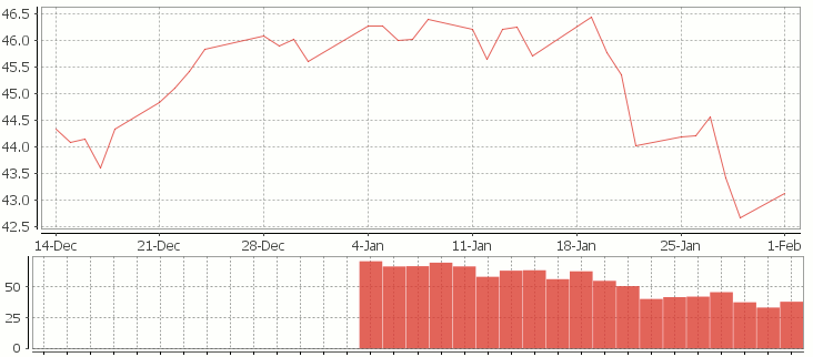
RSI Relative Strength Index stock chart for QQQQ created using qStudio
Or to plot RSI by itself (similar to original article
Writing kdb analytics such as Relative Strength Index is covered in our kdb training course, we offer both public kdb training courses in New York, London, Asia and on-site kdb courses at your offices, tailored to your needs.